1D bar elements

This chapter provides the mathematical foundation for 1D bar and truss elements in femlabpy. We derive the element formulations from continuum mechanics principles, covering both linear and geometrically nonlinear cases.

1. Continuum Mechanics Foundation

1.1 Deformation gradient

Consider a material point at position \(\mathbf{X}\) in the reference configuration that moves to \(\mathbf{x}\) in the current configuration:

\[ \mathbf{x} = \mathbf{X} + \mathbf{u}(\mathbf{X}) \]

The deformation gradient tensor is:

\[ \mathbf{F} = \frac{\partial \mathbf{x}}{\partial \mathbf{X}} = \mathbf{I} + \frac{\partial \mathbf{u}}{\partial \mathbf{X}} \]

For a 1D bar aligned with \(X\), this reduces to the scalar:

\[ F = \frac{dx}{dX} = 1 + \frac{du}{dX} \]

1.2 Strain measures

Engineering strain (small deformation):

\[ \varepsilon = \frac{l - L}{L} = \frac{\Delta L}{L} \]

Green-Lagrange strain (large deformation):

Starting from the definition based on the change in squared length:

\[ E = \frac{1}{2}(F^T F - I) = \frac{1}{2}(C - I) \]

where \(C = F^T F\) is the right Cauchy-Green deformation tensor.

For 1D:

\[ E = \frac{1}{2}(F^2 - 1) = \frac{1}{2}\left[\left(1 + \frac{du}{dX}\right)^2 - 1\right] \]

Expanding:

\[ E = \frac{du}{dX} + \frac{1}{2}\left(\frac{du}{dX}\right)^2 \]

Proof of objectivity: Under rigid body rotation \(\mathbf{Q}\), the deformed configuration transforms as \(\mathbf{x}' = \mathbf{Q}\mathbf{x}\). Then:

\[ \mathbf{F}' = \mathbf{Q}\mathbf{F}, \quad \mathbf{C}' = (\mathbf{F}')^T\mathbf{F}' = \mathbf{F}^T\mathbf{Q}^T\mathbf{Q}\mathbf{F} = \mathbf{F}^T\mathbf{F} = \mathbf{C} \]

Thus \(E' = E\), proving objectivity (frame invariance). ∎

---

2. Linear Bar Element

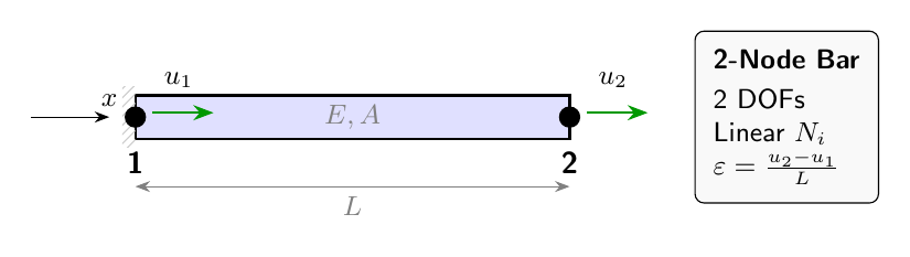
Figure 3.1: Two-node linear bar element with nodal displacements \(u_1\) and \(u_2\).

2.1 Shape functions

For a 2-node element with local coordinate \(\xi \in [0, L]\), the linear shape functions are:

\[ N_1(\xi) = 1 - \frac{\xi}{L}, \quad N_2(\xi) = \frac{\xi}{L} \]

Partition of unity: \(N_1 + N_2 = 1\) for all \(\xi\) ✓

Kronecker delta: \(N_i(\xi_j) = \delta_{ij}\) ✓

The displacement field is interpolated as:

\[ u(\xi) = N_1(\xi) u_1 + N_2(\xi) u_2 = \mathbf{N}(\xi) \mathbf{d}^e \]

2.2 Strain-displacement relation

The strain is the derivative of displacement:

\[\begin{split} \varepsilon = \frac{du}{d\xi} = \frac{dN_1}{d\xi} u_1 + \frac{dN_2}{d\xi} u_2 = \left[-\frac{1}{L}, \frac{1}{L}\right] \begin{bmatrix} u_1 \\ u_2 \end{bmatrix} = \mathbf{B} \mathbf{d}^e \end{split}\]

2.3 Element stiffness derivation

From the principle of virtual work, the internal virtual work equals:

\[ \delta W_{int} = \int_V \delta\varepsilon \, \sigma \, dV = \int_0^L \delta\varepsilon \, E\varepsilon \, A \, d\xi \]

Substituting \(\varepsilon = \mathbf{B}\mathbf{d}^e\):

\[ \delta W_{int} = \delta\mathbf{d}^T \left( \int_0^L A E \, \mathbf{B}^T \mathbf{B} \, d\xi \right) \mathbf{d}^e = \delta\mathbf{d}^T \mathbf{K}^e \mathbf{d}^e \]

Computing the integral:

\[\begin{split} \mathbf{K}^e = AE \int_0^L \begin{bmatrix} 1/L^2 & -1/L^2 \\ -1/L^2 & 1/L^2 \end{bmatrix} d\xi = \frac{EA}{L} \begin{bmatrix} 1 & -1 \\ -1 & 1 \end{bmatrix} \end{split}\]

Symmetry: \(\mathbf{K}^e = (\mathbf{K}^e)^T\) ✓

Positive semi-definiteness: \(\mathbf{d}^T\mathbf{K}^e\mathbf{d} = \frac{EA}{L}(u_1 - u_2)^2 \geq 0\) ✓

---

3. Geometrically Nonlinear Formulation

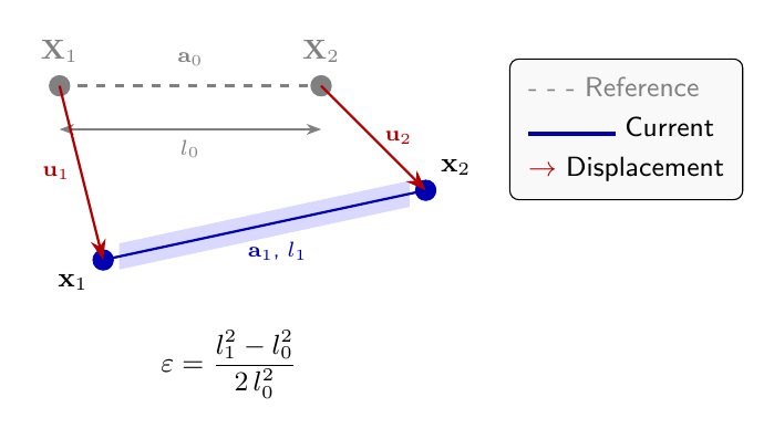
Figure 3.2: Reference and current configurations for Green-Lagrange strain derivation.

3.1 Discrete Green-Lagrange strain

For a bar with initial node positions \(\mathbf{X}_1, \mathbf{X}_2\) and current positions \(\mathbf{x}_1, \mathbf{x}_2\):

\[ \mathbf{a}_0 = \mathbf{X}_2 - \mathbf{X}_1, \quad L_0 = \|\mathbf{a}_0\| \]

\[ \mathbf{a}_1 = \mathbf{x}_2 - \mathbf{x}_1 = \mathbf{a}_0 + \mathbf{u}_2 - \mathbf{u}_1, \quad L_1 = \|\mathbf{a}_1\| \]

The discrete Green-Lagrange strain is:

\[ E = \frac{L_1^2 - L_0^2}{2L_0^2} = \frac{\mathbf{a}_1^T\mathbf{a}_1 - \mathbf{a}_0^T\mathbf{a}_0}{2L_0^2} \]

Linearization: For small displacements, \(L_1 \approx L_0 + \delta L\):

\[ E \approx \frac{(L_0 + \delta L)^2 - L_0^2}{2L_0^2} \approx \frac{\delta L}{L_0} = \varepsilon_{eng} \]

recovering the engineering strain.

3.2 Second Piola-Kirchhoff stress

The work-conjugate stress to Green-Lagrange strain is the Second Piola-Kirchhoff stress:

\[ S = \frac{\partial W}{\partial E} \]

For linear elasticity: \(S = E \cdot \mathcal{E}\) (where \(\mathcal{E}\) is Young’s modulus).

The axial force in the reference configuration is:

\[ N = A_0 S = A_0 E \cdot \mathcal{E} \]

3.3 Virtual work and internal force

The variation of Green-Lagrange strain:

\[ \delta E = \frac{\partial E}{\partial \mathbf{a}_1} \cdot \delta\mathbf{a}_1 = \frac{\mathbf{a}_1^T}{L_0^2} \delta\mathbf{a}_1 \]

Since \(\delta\mathbf{a}_1 = \delta\mathbf{u}_2 - \delta\mathbf{u}_1\):

\[ \delta E = \frac{\mathbf{a}_1^T}{L_0^2} (\delta\mathbf{u}_2 - \delta\mathbf{u}_1) \]

The internal virtual work:

\[ \delta W_{int} = \int_V S \, \delta E \, dV = N L_0 \cdot \delta E = \frac{N}{L_0} \mathbf{a}_1^T (\delta\mathbf{u}_2 - \delta\mathbf{u}_1) \]

This gives the internal force vector:

\[\begin{split} \mathbf{q}^e = \frac{N}{L_0} \begin{bmatrix} -\mathbf{a}_1 \\ \mathbf{a}_1 \end{bmatrix} \end{split}\]

3.4 Tangent stiffness matrix

The tangent stiffness is:

\[ \mathbf{K}_{tan} = \frac{\partial \mathbf{q}^e}{\partial \mathbf{d}^e} \]

Using the product rule on \(\mathbf{q}^e = \frac{N}{L_0}[-\mathbf{a}_1; \mathbf{a}_1]\):

\[\begin{split} \mathbf{K}_{tan} = \underbrace{\frac{1}{L_0}\frac{\partial N}{\partial \mathbf{d}^e}\begin{bmatrix}-\mathbf{a}_1\\\mathbf{a}_1\end{bmatrix}^T}_{\mathbf{K}_m} + \underbrace{\frac{N}{L_0}\frac{\partial}{\partial\mathbf{d}^e}\begin{bmatrix}-\mathbf{a}_1\\\mathbf{a}_1\end{bmatrix}}_{\mathbf{K}_g} \end{split}\]

Material stiffness \(\mathbf{K}_m\):

\[\begin{split} \frac{\partial N}{\partial \mathbf{d}^e} = A\mathcal{E}\frac{\partial E}{\partial \mathbf{d}^e} = \frac{A\mathcal{E}}{L_0^2}\begin{bmatrix}-\mathbf{a}_1^T\\\mathbf{a}_1^T\end{bmatrix} \end{split}\]

Therefore:

\[\begin{split} \mathbf{K}_m = \frac{A\mathcal{E}}{L_0^3} \begin{bmatrix} \mathbf{a}_1\mathbf{a}_1^T & -\mathbf{a}_1\mathbf{a}_1^T \\ -\mathbf{a}_1\mathbf{a}_1^T & \mathbf{a}_1\mathbf{a}_1^T \end{bmatrix} \end{split}\]

Geometric stiffness \(\mathbf{K}_g\):

\[\begin{split} \frac{\partial}{\partial\mathbf{d}^e}\begin{bmatrix}-\mathbf{a}_1\\\mathbf{a}_1\end{bmatrix} = \begin{bmatrix}\mathbf{I} & -\mathbf{I} \\ -\mathbf{I} & \mathbf{I}\end{bmatrix} \end{split}\]

Therefore:

\[\begin{split} \mathbf{K}_g = \frac{N}{L_0} \begin{bmatrix} \mathbf{I} & -\mathbf{I} \\ -\mathbf{I} & \mathbf{I} \end{bmatrix} \end{split}\]

Total tangent:

\[ \mathbf{K}_{tan} = \mathbf{K}_m + \mathbf{K}_g \]

---

4. Mass Matrix

For dynamic analysis, we require the mass matrix relating nodal accelerations to inertial forces.

4.1 Consistent mass matrix

The kinetic energy of a bar element is:

\[ T = \frac{1}{2} \int_0^L \rho A \, \dot{u}^2 \, dx \]

Interpolating \(\dot{u} = \mathbf{N}\dot{\mathbf{d}}^e\):

\[ T = \frac{1}{2} \dot{\mathbf{d}}^T \left( \int_0^L \rho A \, \mathbf{N}^T \mathbf{N} \, dx \right) \dot{\mathbf{d}} = \frac{1}{2} \dot{\mathbf{d}}^T \mathbf{M}^e \dot{\mathbf{d}} \]

Computing the integral:

\[\begin{split} \mathbf{M}^e = \rho A \int_0^L \begin{bmatrix} N_1^2 & N_1 N_2 \\ N_1 N_2 & N_2^2 \end{bmatrix} dx \end{split}\]

Using \(N_1 = 1 - \frac{x}{L}\) and \(N_2 = \frac{x}{L}\):

\[ \int_0^L N_1^2 \, dx = \frac{L}{3}, \quad \int_0^L N_2^2 \, dx = \frac{L}{3}, \quad \int_0^L N_1 N_2 \, dx = \frac{L}{6} \]

Proof of \(\int_0^L N_1^2 dx = L/3\):

\[ \int_0^L \left(1 - \frac{x}{L}\right)^2 dx = \int_0^L \left(1 - \frac{2x}{L} + \frac{x^2}{L^2}\right) dx = \left[x - \frac{x^2}{L} + \frac{x^3}{3L^2}\right]_0^L = L - L + \frac{L}{3} = \frac{L}{3} \quad \checkmark \]

Therefore the consistent mass matrix is:

\[\begin{split} \mathbf{M}^e_{cons} = \frac{\rho A L}{6} \begin{bmatrix} 2 & 1 \\ 1 & 2 \end{bmatrix} \end{split}\]

4.2 Lumped mass matrix

The lumped mass matrix concentrates mass at the nodes:

\[\begin{split} \mathbf{M}^e_{lump} = \frac{\rho A L}{2} \begin{bmatrix} 1 & 0 \\ 0 & 1 \end{bmatrix} \end{split}\]

Conservation property: Both formulations preserve total mass:

\[ \text{trace}(\mathbf{M}_{cons}) = \frac{\rho A L}{6}(2 + 2) = \frac{2\rho A L}{3} \neq \rho A L \]

Wait—the consistent matrix does not preserve total mass per DOF. However, the sum of all entries equals \(\rho A L\) in both cases:

\[ \sum_{ij} M^{cons}_{ij} = \frac{\rho A L}{6}(2 + 1 + 1 + 2) = \rho A L \quad \checkmark \]

---

5. Transformation to Global Coordinates

For 2D/3D trusses, the local stiffness must be transformed to global coordinates.

5.1 Rotation matrix

Let \(\mathbf{e}\) be the unit vector along the bar from node 1 to node 2:

\[ \mathbf{e} = \frac{\mathbf{X}_2 - \mathbf{X}_1}{L_0} \]

In 2D, \(\mathbf{e} = [\cos\theta, \sin\theta]^T\) where \(\theta\) is the angle with the global \(x\)-axis.

The transformation matrix \(\mathbf{T}\) relates local DOFs to global DOFs:

\[ \mathbf{d}^{local} = \mathbf{T} \mathbf{d}^{global} \]

For 2D:

\[\begin{split} \mathbf{T} = \begin{bmatrix} \cos\theta & \sin\theta & 0 & 0 \\ 0 & 0 & \cos\theta & \sin\theta \end{bmatrix} \end{split}\]

5.2 Stiffness transformation

The global stiffness is obtained via congruent transformation:

\[ \mathbf{K}^{global} = \mathbf{T}^T \mathbf{K}^{local} \mathbf{T} \]

Proof of symmetry preservation: If \(\mathbf{K}^{local}\) is symmetric:

\[ (\mathbf{K}^{global})^T = (\mathbf{T}^T \mathbf{K}^{local} \mathbf{T})^T = \mathbf{T}^T (\mathbf{K}^{local})^T \mathbf{T} = \mathbf{T}^T \mathbf{K}^{local} \mathbf{T} = \mathbf{K}^{global} \quad \checkmark \]

---

6. Implementation Reference

Element force: qebar

import numpy as np

def qebar(Xe0, Xe1, Ge):
    """Internal force vector for geometrically nonlinear bar."""
    a0 = (Xe0[1] - Xe0[0]).reshape(-1, 1)
    L0 = float(np.linalg.norm(a0))
    a1 = (Xe1[1] - Xe1[0]).reshape(-1, 1)
    L1 = float(np.linalg.norm(a1))

    A, E = Ge[0], Ge[1]
    
    # Green-Lagrange strain
    strain = 0.5 * (L1**2 - L0**2) / L0**2
    stress = E * strain
    
    # Internal force vector
    qe = (A * stress / L0) * np.vstack([-a1, a1])
    return qe, stress, strain

Tangent stiffness: kebar

def kebar(Xe0, Xe1, Ge):
    """Tangent stiffness for geometrically nonlinear bar."""
    a0 = (Xe0[1] - Xe0[0]).reshape(-1, 1)
    L0 = float(np.linalg.norm(a0))
    a1 = (Xe1[1] - Xe1[0]).reshape(-1, 1)

    A, E = Ge[0], Ge[1]
    
    strain = 0.5 * (np.linalg.norm(a1)**2 - L0**2) / L0**2
    N = A * E * strain
    
    I = np.eye(a0.shape[0])
    
    K_m = (E * A / L0**3) * np.block([
        [ a1 @ a1.T, -a1 @ a1.T],
        [-a1 @ a1.T,  a1 @ a1.T]
    ])
    
    K_g = (N / L0) * np.block([
        [ I, -I],
        [-I,  I]
    ])
    
    return K_m + K_g